
How our Tax Coordination feature can boost your returns
Our spin on asset location can help shelter retirement investment growth from some taxes.


Taxes. You may try to think of them as little as possible, but they’re on our minds a lot. Especially when they relate to investments. That’s because we’re always looking to maximize our customers’ potential take-home returns—and key to that pursuit is minimizing how big of a bite taxes take.
On that front, our Tax Coordination feature is a fully-automated approach to an investment strategy known as asset location—and it’s available at no additional cost. If you’re saving for retirement in more than one type of account, then asset location in general, and our spin on it specifically, can help to increase your after-tax expected returns without taking on additional risk. Here’s how.
How Tax Coordination works
Many Americans wind up saving for retirement in some combination of three account types:
- Taxable
- Tax-deferred (Traditional 401(k) or IRA)
- Tax-exempt (Roth 401(k) or Roth IRA)
Each type of account gets a different tax treatment, and different assets are taxed differently as well. These rules make certain investments a better fit for one account type over another.
Returns in IRAs and 401(k)s, for example, don’t get taxed annually, so they generally shelter growth from tax better than a taxable account. We’d rather shield assets that lose more to tax in these types of retirement accounts, assets such as bonds, whose dividends are usually taxed annually and at a high rate.
In the taxable account, however, we’d generally prefer to have assets that don’t get taxed as much, assets such as stocks, whose growth in value (“capital gains”) is taxed at a lower rate and crucially only when they’re “realized,” or in other words, when they’re sold at a higher price than what you paid for them.
Wisely applying this strategy to a globally-diversified portfolio can get complicated quickly. Check out our full Asset Location methodology if you’re curious what that complexity looks like—or keep reading for more of the simplified explanation.
The big picture diversification of asset location
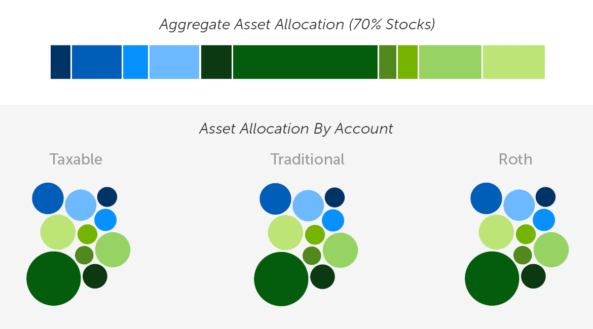
When investing in more than one account, many people select the same portfolio in each one. This is easy to do, and when you add everything up, you get the same portfolio, only bigger.
To illustrate this approach, here’s what it looks like with a hypothetical asset allocation of 70% stocks and 30% bonds. The different shades of green represent various types of stocks, and the different shades of blue represent various types of bonds.
But as long as all the accounts add up to the portfolio we want, each individual account on its own doesn’t have to mirror that portfolio. Each asset can go in the account where it makes the most sense from a tax perspective. As long as we still have the same portfolio when we add up the accounts, we can increase the after-tax expected return without taking on more risk. This is asset location in action, and here’s what it looks like, again for illustrative purposes: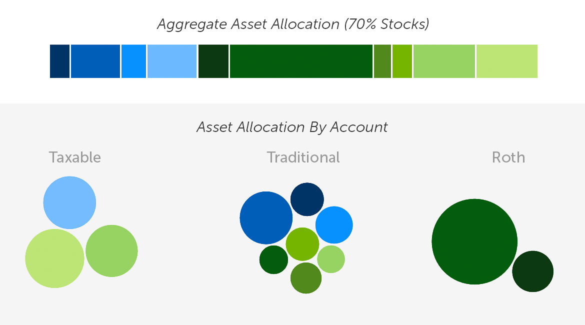
This is the same overall portfolio as we originally showed, except we redistributed the assets unevenly to reduce taxes. Note that the aggregate allocation is still a 70/30 split of stocks and bonds.
The concept of asset location isn’t new. Advisors and sophisticated do-it-yourself investors have been implementing some version of this strategy for years. But squeezing it for more benefit is very mathematically-complex. It means making necessary adjustments along the way, especially after making deposits to any of the accounts. Our expert-built technology handles all of the complexity in a way that a manual approach just can’t match.
Our rigorous research and testing, as outlined in our Asset Location methodology, demonstrates that accounts managed by Tax Coordination are expected to yield meaningfully higher after-tax returns than uncoordinated accounts.
How to benefit from Betterment’s Tax Coordination
To benefit from from our Tax Coordination feature, you first need to be a Betterment customer with a balance in at least two of the following types of Betterment accounts:
- Taxable account
- Tax-deferred account: A Traditional IRA or a Betterment Traditional 401(k) offered by your employer.
- Tax-exempt account: A Roth IRA or a Betterment Roth 401(k) offered by your employer.
Note that you can only include a 401(k) in a goal using Tax Coordination if it’s one we manage on behalf of your current or former employer. If your employer doesn’t currently use Betterment to provide their 401(k) plan, tell them to give us a look at betterment.com/work!
If you have an old 401(k) with a previous employer, you can still benefit from our Tax Coordination feature by rolling it over to a Betterment IRA.
For step-by-step instructions on how to set up Tax Coordination in your Betterment account, as well as answers to frequently asked questions, head on over to our Help Center. Or if you’re not yet a Betterment customer, get started by signing up today.
